DNN 분류 (DNN Classification)
이번 포스팅에서는 DNN을 사용하여 "패션 이미지 데이터를 분류하는 방법"과 "텍스트 데이터를 감성분석하는 방법"을 알아보겠습니다.
DNN 이미지 분류 (DNN Image Classification)
Fashion MNIST(MNIST) Dataset
10개의 범주(category)와 70,000개의 흑백 이미지로 구성된 패션 MNIST 데이터셋.
이미지는 해상도(28x28 픽셀)가 낮고 다음처럼 개별 의류 품목을 나타낸다:
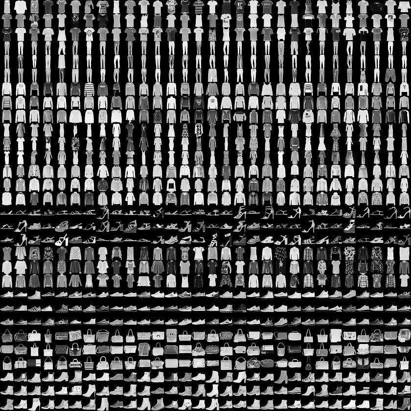
패션 MNIST와 손글씨 MNIST는 비교적 작기 때문에 알고리즘의 작동 여부를 확인하기 위해 사용되곤 하며 코드를 테스트하고 디버깅하는 용도로 좋다.
이미지는 28x28 크기의 넘파이 배열이고 픽셀 값은 0과 255 사이이다. 레이블(label)은 0에서 9까지의 정수 배열이다. 아래 표는 이미지에 있는 의류의 클래스(class)를 나낸다.
| 레이블 | 클래스 |
|---|---|
| 0 | T-shirt/top |
| 1 | Trouser |
| 2 | Pullover |
| 3 | Dress |
| 4 | Coat |
| 5 | Sandal |
| 6 | Shirt |
| 7 | Sneaker |
| 8 | Bag |
| 9 | Ankle boot |
각 이미지는 하나의 레이블에 매핑되어 있다. 데이터셋에 클래스 이름이 들어있지 않기 때문에 나중에 이미지를 출력할 때 사용하기 위해 별도의 변수를 만들어 저장한다.
Data Setting
class_names = ['T-shirt/top', 'Trouser', 'Pullover', 'Dress', 'Coat', 'Sandal', 'Shirt', 'Sneaker', 'Bag', 'Ankle boot']import numpy as np
import tensorflow as tf
import tensorflow.keras as keras
np.random.seed(1)
tf.random.set_seed(1)# 데이터셋 읽이어기
(X_train, y_train), (X_test, y_test) = keras.datasets.fashion_mnist.load_data()
X_train.shape, y_train.shape # ((60000, 28, 28), (60000,))
X_test.shape, y_test.shape # ((10000, 28, 28), (10000,))
item, counts = np.unique(y_train, return_counts=True)
dict(zip(item, counts))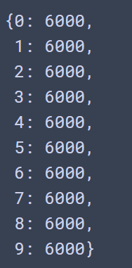
item, counts = np.unique(y_test, return_counts=True)
dict(zip(item, counts))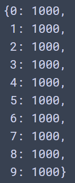
import matplotlib.pyplot as plt
plt.imshow(X_train[0], cmap='Greys')
plt.colorbar()
plt.show()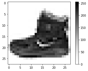
DNN 모델링을 위한 데이터 전처리
# 하이퍼파라미터
learning_rate = 0.001
N_EPOCHS = 30
N_BATCH = 100
N_CLASS = 10 # 라벨의 개수
N_TRAIN = X_train.shape[0] #학습 데이터 수
N_TEST = X_test.shape[0]   #테스트 데이터 수
# 데이터 전처리
# X : 0 ~ 1사이로 scaling
X_train = X_train/255
X_test = X_test/255
# y를 원핫인코딩
y_train = keras.utils.to_categorical(y_train, N_CLASS)
y_test = keras.utils.to_categorical(y_test, N_CLASS)
print(y_train [:2])
# [[0. 0. 0. 0. 0. 0. 0. 0. 0. 1.]
[1. 0. 0. 0. 0. 0. 0. 0. 0. 0.]]train_dataset = tf.data.Dataset.from_tensor_slices((X_train,y_train))\
.shuffle(100000)\
.batch(N_BATCH, drop_remainder=True).repeat()
test_dataset = tf.data.Dataset.from_tensor_slices((X_test, y_test)).batch(N_BATCH)
DNN Image Classification 모델링 및 성능평가
# 모델 생성
def create_model():
    model = keras.Sequential()
    # 레이어 추가
    model.add(keras.layers.Flatten(input_shape=(28,28)))  #height/width
    model.add(keras.layers.Dense(256, activation='relu'))
    model.add(keras.layers.Dense(128, activation='relu'))
    model.add(keras.layers.Dense(64, activation='relu'))
    #출력층 - multi class 분류: units수-class수, activation-softmax
    model.add(keras.layers.Dense(N_CLASS, activation='softmax'))

    return model
# 모델 생성, 컴파일
model = create_model()
# loss함수: multiclass 분류 - categorical_crossentropy
model.compile(optimizer=tf.keras.optimizers.Adam(learning_rate),
loss='categorical_crossentropy', metrics=['accuracy'])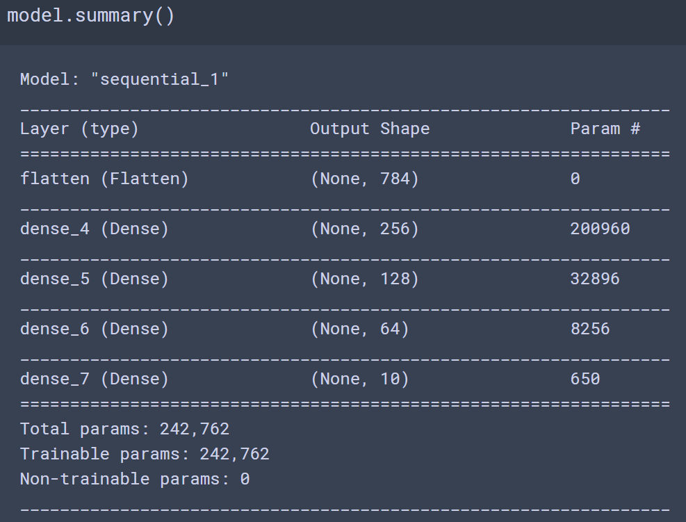
steps_per_epoch = N_TRAIN // N_BATCH
validation_steps = int(np.ceil(N_TEST/N_BATCH))

# 학습
history = model.fit(train_dataset, epochs=N_EPOCHS, steps_per_epoch=steps_per_epoch,
                    validation_data=test_dataset, validation_steps=validation_steps)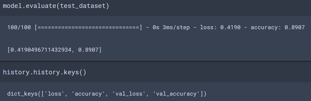
# loss
plt.figure(figsize=(10,7))

plt.plot(history.history['loss'], label='Train loss')
plt.plot(history.history['val_loss'], label='Validation loss')

plt.title("Loss")
plt.legend()
plt.show()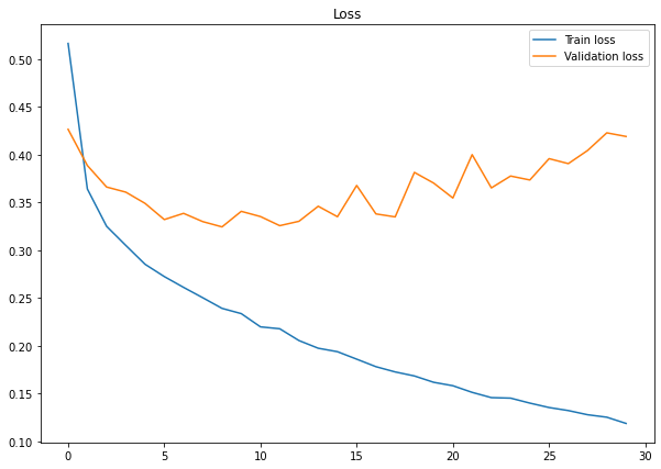
plt.figure(figsize=(10,7))

plt.plot(history.history['accuracy'], label='Train accuracy')
plt.plot(history.history['val_accuracy'], label='Validation accuracy')

plt.title("accuracy")
plt.legend()
plt.show()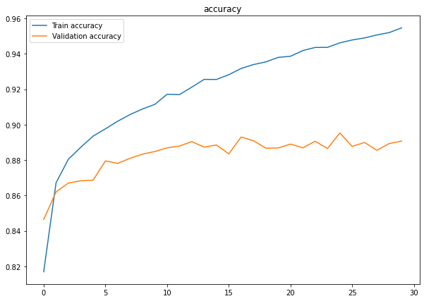
DNN 감성분석 (DNN Sentiment Analysis Classification)
IMDB Dataset
- class: 0-부정리뷰, 1-긍정리뷰
- pkl파일 : 텍스트 전처리까지 한 것 (텍스트 마이닝 IMDB 감정분석 참고)
import numpy as np
import tensorflow as tf
import tensorflow.keras as keras
import pickle
import matplotlib.pyplot as plt

np.random.seed(1)
tf.random.set_seed(1)


# 데이터 읽기
with open('imdb_text_preprocess_data/X_train.pkl', 'rb') as f:
    X_train = pickle.load(f)

with open('imdb_text_preprocess_data/y_train.pkl', 'rb') as f:
    y_train = pickle.load(f)

with open('imdb_text_preprocess_data/X_test.pkl', 'rb') as f:
    X_test = pickle.load(f)

with open('imdb_text_preprocess_data/y_test.pkl', 'rb') as f:
    y_test = pickle.load(f)
# 벡터화
from sklearn.feature_extraction.text import TfidfVectorizer
tfidf = TfidfVectorizer()
X_train = tfidf.fit_transform(X_train).toarray()
X_test = tfidf.transform(X_test).toarray()
X_train.shape, y_train.shape, X_test.shape, y_test.shape # ((25000, 48956), (25000,), (25000, 48956), (25000,))DNN 모델링을 위한 데이터 세팅
# 하이퍼라파미터
learning_rate = 0.001
N_EPOCHS = 10
N_BATCH = 100

N_TRAIN = X_train.shape[0]
N_FEATURES = X_train.shape[1]
N_TEST = X_test.shape[0]

# 데이터셋 구성
train_dataset = tf.data.Dataset.from_tensor_slices((X_train, y_train))\
                               .shuffle(N_TRAIN)\
                               .batch(N_BATCH, drop_remainder=True).repeat()

test_dataset = tf.data.Dataset.from_tensor_slices((X_test, y_test))\
                              .batch(N_BATCH)
DNN 모델링 및 성과평가
# 모델 구성
def create_model():
    model = keras.Sequential()
    #입력층
    model.add(keras.layers.Dense(512, activation='relu', input_shape=(N_FEATURES,)))
    model.add(keras.layers.Dense(256, activation='relu'))
    model.add(keras.layers.Dense(256, activation='relu'))
    model.add(keras.layers.Dense(256, activation='relu'))
    #출력층 - 이진분류(binary classification): units-1, actitvation-sigmoid
    model.add(keras.layers.Dense(1, activation='sigmoid'))

    return model
# 모델생성, 컴파일
model = create_model()
# 이진분류 - loss : binary_crossentropy
model.compile(optimizer=keras.optimizers.Adam(learning_rate),
loss='binary_crossentropy',
metrics=['accuracy'])
steps_per_epoch = N_TRAIN//N_BATCH
validation_steps = int(np.ceil(N_TEST/N_BATCH))# 학습
history = model.fit(train_dataset, epochs=N_EPOCHS, steps_per_epoch=steps_per_epoch,
validation_data = test_dataset, validation_steps=validation_steps)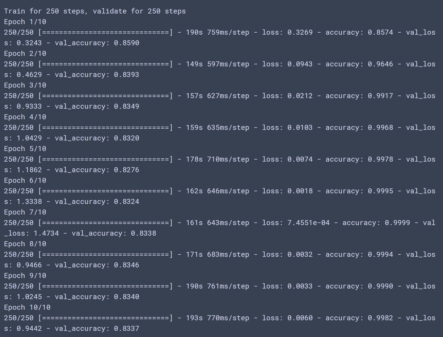
plt.figure(figsize=(10,7))
plt.plot(history.history['loss'], label='Train loss')
plt.plot(history.history['val_loss'], label='Validation loss')
plt.title('Loss')
plt.legend()
plt.show()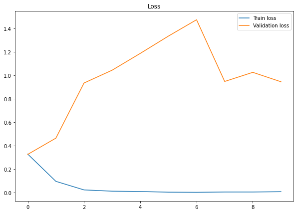
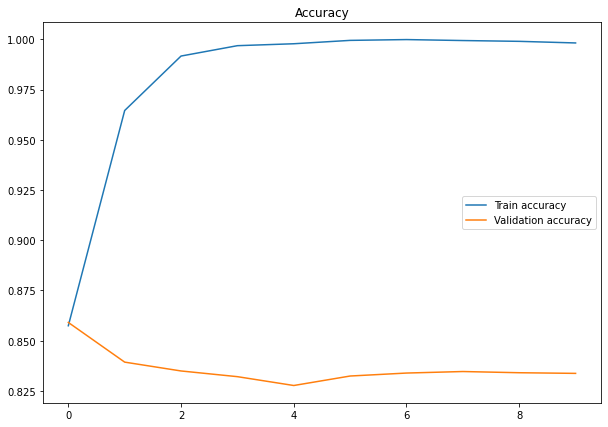
plt.figure(figsize=(10,7))
plt.plot(history.history['accuracy'], label='Train accuracy')
plt.plot(history.history['val_accuracy'], label='Validation accuracy')
plt.title('Accuracy')
plt.legend()
plt.show()
728x90
반응형
'Data Analysis & ML > Deep Learning' 카테고리의 다른 글
| [Deep Learning][딥러닝] CNN 개요 (0) | 2020.11.09 |
|---|---|
| [Deep Learning][딥러닝] DNN 성능개선 (0) | 2020.11.09 |
| [Deep Learning] DNN 회귀분석 (Tensorflow Dataset) (0) | 2020.09.23 |
| [Deep Learning] DNN (Deep Neural Network) (0) | 2020.09.22 |
| [Deep Learning][딥러닝] 딥러닝 구현 (0) | 2020.09.22 |