MNIST 데이터에 CNN 적용
하이퍼파라미터 및 데이터셋 전처리
import tensorflow as tf
import tensorflow.keras as keras
import tensorflow.keras.layers as layers
import numpy as np
np.random.seed(1)
tf.random.set_seed(1)
# 하이퍼파라미터 정의
learning_rate = 0.001
N_EPOCHS = 20
N_BATCH = 100
N_CLASS = 10# 데이터 저장
(train_images, train_labels), (test_images, test_labels) = keras.datasets.mnist.load_data()N_TRAIN = train_images.shape[0]
N_TEST = test_images.shape[0]
train_images.shape, test_images.shape
#(개수, height, width, channel) => ((60000, 28, 28), (10000, 28, 28))# 전처리 - image-0 ~ 1사이로 조정
X_train = train_images/255
X_test = test_images/255
# X의 차원을 3차원->4차원으로 변경. (channel 추가)
# (60000,28,28) => (60000,28,28, 1)
X_train = X_train[..., np.newaxis]
X_test = X_test[..., np.newaxis]
X_train.shape, X_test.shape
# ((60000, 28, 28, 1), (10000, 28, 28, 1))# y를 one hot encoding => 활성화함수를 적용하려면 y가 0과 1로 이루어져있어야 한다.
print(train_labels[:5])
y_train = keras.utils.to_categorical(train_labels, N_CLASS)
y_test = keras.utils.to_categorical(test_labels, N_CLASS)
print(y_train[:5])# Dataset 구성(train, test 데이터셋 구성)
train_dataset = tf.data.Dataset.from_tensor_slices((X_train, y_train))\
.shuffle(N_TRAIN)\
.batch(N_BATCH, drop_remainder=True).repeat()
test_dataset = tf.data.Dataset.from_tensor_slices((X_test, y_test)).batch(N_BATCH)모델 구성
# 모델 구성 CNN - Conv, Pooling , Dense
def create_model():
    model = keras.Sequential()
    # Feature Extraction -> Convolution + Pooling layer
    # Conv2D(Convolution Layer) + input_shape 지정(height, width, channel)
    model.add(layers.Conv2D(filters=32, #필터개수 (1개의 필터가 1개의 특성 찾는다.)
                            kernel_size=3, #필터의 크기. (3,3) height,width가 같은 경우 하나만 써준다.
                            padding='SAME',# 패딩방식-SAME,VALID (대소문자 상관없다.)
                            strides=1,  #얼만큼씩 이동할지 지정. default: (1,1)
                            activation='relu',
                            input_shape=(28,28,1)))
    # MaxPooling Layer
    model.add(layers.MaxPool2D(pool_size=2,  #size: default=(2,2)
                               strides=2, #기본값: None=>pool size와 동일
                               padding='SAME'))

    model.add(layers.Conv2D(filters=64, kernel_size=3, padding='SAME', activation='relu'))
    model.add(layers.MaxPool2D(padding='SAME'))

    model.add(layers.Conv2D(filters=128, kernel_size=3, padding='SAME', activation='relu'))
    model.add(layers.MaxPool2D(padding='SAME'))
    # Classification Layers => Fully Connected Layers
    model.add(layers.Flatten())
    model.add(layers.Dense(256, activation='relu'))
    model.add(layers.Dropout(0.4))
    #출력 layer
    model.add(layers.Dense(N_CLASS, activation='softmax'))

    return model
# 모델생성 및 컴파일
model = create_model()
model.compile(optimizer=keras.optimizers.Adam(learning_rate),
loss='categorical_crossentropy',
metrics=['accuracy'])
model.summary()
# 학습전에 모델 평가
model.evaluate(test_dataset) #loss: 2.3034 - accuracy: 0.0974

# loss 가 np.log(클래스수) 보다 크면(많이 차이가 나면) 모델을 수정한다.
np.log(N_CLASS) #2.302585092994046
steps_per_epoch = N_TRAIN//N_BATCH
validation_steps = int(np.ceil(N_TEST/N_BATCH))
history = model.fit(train_dataset, epochs=N_EPOCHS, steps_per_epoch=steps_per_epoch,
                    validation_data=test_dataset, validation_steps=validation_steps)
모델 평가
import matplotlib.pyplot as plt
# 학습결과 그래프 함수
# loss 그래프
def loss_plot(history):
#     plt.figure(figsize=(10,7))
    plt.plot(history.history['loss'], label='Train loss')
    plt.plot(history.history['val_loss'], label='Validation loss')
    plt.title('Loss')
    plt.xlabel('Epoch')
    plt.ylabel('Loss')
    plt.legend()
    plt.show()

# accuracy 그래프
def accuracy_plot(history):
#     plt.figure(figsize=(10,7))
    plt.plot(history.history['accuracy'], label='Train accuracy')
    plt.plot(history.history['val_accuracy'], label='Validation accuracy')
    plt.title('accuracy')
    plt.xlabel('Epoch')
    plt.ylabel('accuracy')
    plt.legend()
    plt.show()
loss_plot(history)
accuracy_plot(history)
Prediction Error(예측 오차)가 발생한 example 확인
# test set을 예측
test_pred = model.predict_classes(X_test)

# 실제 label과 예측 결과 비교
error_idx = np.where(np.not_equal(test_labels, test_pred))[0]
error_idx
# 틀린것들 label비교(10개만)
for idx in error_idx[:10]:
    print((test_labels[idx], test_pred[idx]))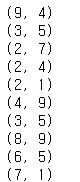
plt.figure(figsize=(30,10))
for i in range(10):
    idx = error_idx[i]
    plt.subplot(1,10, i+1)
    plt.imshow(test_images[idx], cmap='Greys')
    plt.xticks([])
    plt.yticks([])
plt.show(
728x90
반응형
'Data Analysis & ML > Deep Learning' 카테고리의 다른 글
| [Deep Learning] 모델 저장하는 방법 (HDF5/tensorflow SaveModel/Callback) (0) | 2021.01.24 |
|---|---|
| [Deep Learning][딥러닝] CNN Image Augmentation(이미지 증식) (0) | 2021.01.24 |
| [Deep Learning][딥러닝] CNN_MNIST분류 / 모델저장/ FunctionalAPI (0) | 2020.11.09 |
| [Deep Learning][딥러닝] CNN 개요 (0) | 2020.11.09 |
| [Deep Learning][딥러닝] DNN 성능개선 (0) | 2020.11.09 |